Hungarian Method : Perfect Matching – Min Cost
Finding Optimal Matchings
Daily life contains many problems that can be modeled using matchings in bipartite graphs. Here, we consider weighed proglems in particular
Let’s look at the following problem as an example: An CEO is faced with a multitude of tasks that have to be dealt with in his company. However, his employees have diverse qualifications and certain tasks suit some employees more than others. This means that a certain level of efficiency will be assigned for each employee performing a certain task. The CEO obviously wants his company to run as efficiently as possible, thus he has to assign tasks to employees in such a way that the level of efficiency is maximized (to the extend possible) for each task.
We can model this problem as a bipartite graph with vertex sets (orange) representing the employees and (red) representing the tasks (see Figure 1). All the following illustrations will use these labelings. The weighed edges between these sets then define the total number of hours that employee will need to complete task . The goal is to find a perfect matching that minimizes the sum of edge weights.
The Hungarian Method
The problem can be solved using the Hungarian Method that was developed in 1955 by Harold W. Kuhn based on the ideas of two hungarian mathematicians (Dénes Kőnig and Jenő Egerváry). Later, the algorithm was improved by James Munkres. It’s based on a central theorem. In order to understand this, we will have to introduce some concepts:
Labels
We introduce a simple helper function or label , that assigns a real number to each vertex in the graph, such that the sum of the labels of two edges is at least as great thatn the weight of the edge that connect these vertices (see Figure 2).
Equality Graph
Using these labels, we can construct an equality graph that contains all nodes from the original Graph. However, the edge set will only contain those edges that have exactly the weight of the sum of the labels of their corresponding vertices (Figure 3).
Now back to the theorem mentioned above: The Kuhn-Munkres theorem states that any perfect matching in the equality graph is maximal in the original graph. Thus, the problem of finding an optimal matching can be reduced to finding a perfect matching in the equality graph.
Some more information before we look at the algorithm itself:
The Hungarian Method as described here will find maximal matchings, meaning matchings with their total edge weights as great as possible. This implies that we will have to remodel the problem described in the beginning: To do so, we “mirror” the edge weights by changing the sign, i.e. turning into .
Furthermore, the bipartite graph that we run the algorithm on must be complete, thus the number of nodes in and must be the same and there must be an edge between any two vertices that lie in different partitions. In our example, this would not be the case, if some employee is not qualified to work on some specific job. In this case, we will introduce neutral vertices and edges with weight , such that the graph becomes complete. If any of the neutral elements are contained in the matching that the algorithm ultimately finds, we can simply remove them again.
The Execution of the Algorithm
The algorithm uses an iterative approach for finding a perfect matching in the equality graph. It starts with an empty matching and tries to improve the current matching in every step, until perfection is reached.
In the beginning, the algorithm specifies a label for each node. Every node in is assigned the weight of its heaviest edge, each vertex in begins with the label . Using these labels, the algorithm then constructs the equality graph. For the next steps, we must first introduce some more concepts:
Alternating and Augmenting Paths
We call a vertex matched, iff it has an edge that is contained in the current matching; otherwise we call it free (compare Figure 4).
An alternating path is a sequence of edges where the edges alternate between being contained and not contained in the matching . An alternating path is called augmenting, if both its origin and destination nodes are free (see Figure 6).
In order to improve on the existing (still empty) matching, the algorithm selects a node in that does not yet have a matching partner. Starting in this node, we then look for an augmenting path: In order to do this, the algorithm builds up an alternating path step by step, until the path either becomes augmenting or no further qualified edges exist. We partition the nodes that have been visited by this procedure into the sets for visited nodes in and for nodes in , respectively.
However, it is not always possible to find an augmenting path. If this is the case, the algorithm must improve the labels assigned to the vertices. The improvement must be performed in a way such that the current matching is preserved in the equality graph. Furthermore, the equality graph must be extended with additional edges in such a way that a new alternating path can be constructed. This can be insured by first specifying a value by considering all pairs of visited nodes and unvisited nodes and calculating the minimum of the sum of their respective labels minus the weight of the edge between them.
The labels of all nodes can now be adjusted using before defining the new equality graph and in turn surching for augmenting paths.
If the path does find an augmenting path, it improves on the current matching by adding the edges of the path which are not currently contained in the matching and removing those from the path that currently are. This step is being repeated until each node has a matching partner and the matching is thus perfect. Using the theorem given above, the matching found in this way must then be maximal in terms of edge weights.
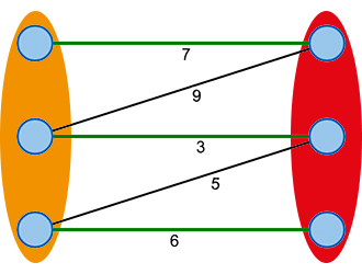
Figure 1: An optimal matching (green)
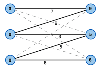
Figure 2: Node markings
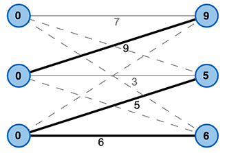
Figure 3: Equality Graph
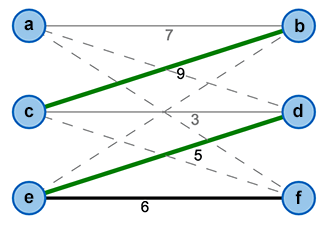
Figure 4: Free (a,f) and Matched Nodes (b,c,d,e)
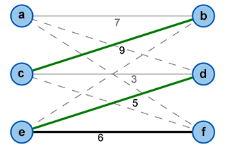
Figure 5: An Alternating Path (f,e,d)
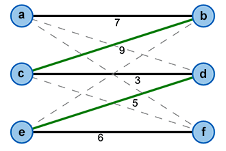
Figure 6: An Augmenting Path (f,e,d,c,b,a)