Matching on bipartite Graphs

Numerous allocation problems can be modeled as bipartite matching problems. A simple example is the matching of students to open job positions. Not every assignment is possible as students will differ in their qualifications. The problem can be made easier to grasp if you consider the students to be a set of vertices and the jobs as another set of vertices. The edges between these sets will then represent all valid assignments of a student to a job. The goal is to find as many valid assignments as possible, while each student may only take one job and each job can be assigned to only a single student.

Let  be a given bipartite graph. A graph is called bipartite if it consists of two sets of vertices U and V, such that no edges exist within these sets. A matching is a set of edges, such that every vertex lies on at most one of the edges in this set. Figure 1 shows a matching in a bipartite graph. The problem we investigate is to find a mathching on G with maximal cardinality (i.e. maximal number of elements).

Idea of the Algorithm

Let M be the current matching (starting with the empty set). We will call an edge a matching edge if it is contained in M, and a free edge otherwise. In the illustrations, free and matching edges are shown in black and green, respectively. A node that lies on a matching edge is called covered (or matched). Otherwise the vertex is free. Covered nodes are shown in green, free nodes in blue. An augmenting path in the graph G is a path that

• starts in a free node,
• ends in a free node, and
• alternates between free and matching edges.

Figure 2 illustrates an augmenting path in a graph.

Consider an augmenting path. If we remove all its matching edges from M, but add all its free edges, then the cardinality of M will increase by exactly 1. All nodes on the augmenting path lie on at most one matching edge. The end nodes of the path are not part of any matching edge, therefore we get a valid matching again after augmentation. The number of free edges in any augmenting path is exactly the number of matching edges plus 1. Thus the matching will be enlarged after augmentation.

A theorem in Graph Theory states the following:
A matching M in G(V,E) is maximal (w.r.t. cardinality) iff (if and only if) no augmenting paths exist.
A simple algorithm to find maximal matchings is thus to search for an augmenting path and increase the size of the matching along it. If no more augmenting paths can be found, the matching is optimal. However, the running time of this algorithm can be quite long in some cases.

The algorithm by Hopcroft and Karp improves the runtime when compared to the simple algorithm above. In each iteration, it only considers the shortest augmenting paths, and looks for a set of vertex-disjunct augmenting paths, i.e. no two such paths can share a node.

The set of shortest vertex-disjunct augmenting paths should be inclusion-maximal. This means that no other augmenting path exists that is vertex-disjunct to the paths already contained in the set. After finding the inclusion-maximal set of augmenting paths, we augment the matching and start a new iteration. After each iteration, the length of the shortest augmenting path will increase. The proof for this is somewhat complicated and will be ommitted here. However, it should be intuitive that the length of augmenting paths cannot become shorter after an augmentation. If no more augmenting paths exist, the algorithm terminates.

Finding Shortest Augmenting Paths

The shortest augmenting paths can be found using Breadth-first (BFS) und Depth-first search (DFS). We start with all free nodes in an (arbitrary) set of vertices and add these to the first layer of a layered graph, that will represent a decomposition of V into multiple layers and will be explained in more detail in the following. The layered graph will be created iteratively, until a free node has been found or all nodes have already been checked. The layered graph is constructed using the following procedure:

Starting from the nodes of the current layer one follows all edges to neighbors that haven’t been considered yet. These neighbors make up the next layer of the graph. If this new layer contains a free node, the procedure will terminate; if the layer is empty, it will terminate as well and return that no further augmenting paths exist. Otherwise the layered graph will be extended by another layer, using the matching parners of the nodes in the previous layer. This layer of matching partners then becomes the current layer and the procedure is repeated until it terminates (see above). Finally, we end up with a layered graph that contains all (and only the) shortest augmenting paths, if any such paths exist.

The third figure shows a layered graph with four layers. The first layer consists of two free nodes from the vertex set above. Their neighbors are added to the second layer. Since none of the nodes in the second layer are free, a third layer is added, comprising the matching partners of the nodes in the second layer. All neighbors of this third layer that have not been considered yet are finally added to the fourth layer. As two of these vertices are free, the procedure ends after four layers.

Now, we use the layered graph from the last stet to find an inclusion-maximal set of vertex-disjunct augmenting paths. We use a Depth-first search starting with the free nodes in the first layer. If there is an augmenting path starting in one of these nodes, then it will be found. All nodes that are being used in this path will be deleted from the layered graph, or highlighted. While executing the algorithm, these nodes will be marked in gray. Applying this procedure to all nodes of the first layer, the set of shortest augmenting paths found this way will be vertex-disjunct, and after termination of the procedure no other augmenting paths will exist that is vertex-disjunct with respect to those already found.

In Figure three, the vertex-disjunct augmenting paths are highlighted by bold arrows. Thus, in this iteration the algorithm would augment the matching using these two augmenting paths. Afterwars a new iteration would begin and a new layered graph would be constructed.

The advantage of the layered graph is that all shortest augmenting paths can be found simultaneously. In the worst case, we have to check all edges in order to specify an inclusion-maximal set of shortest, vertex-disjunct augmenting paths.

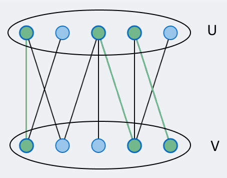
Figure 1
Matching in a bipartite graph

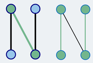
Figure 2
Simple graph with an augmenting path.
On the left, an augmenting path has been highlightet. On the right, you see the graph after the augmentation.

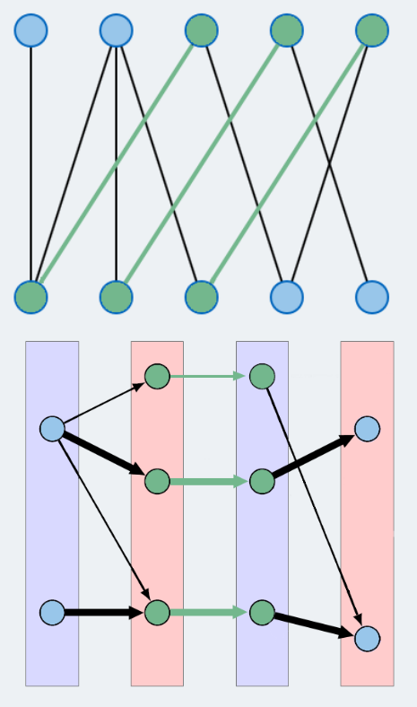
Figure 3
Graph with its corresponding layered graph.
The vertex-disjunct augmenting paths are highlighted in the layered graph.

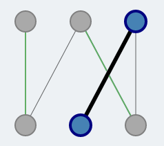
Figure 4
The gray vertices are already included in other shortest augmenting paths in this iteration. The highlighted agumentation path is vertex-disjunct to all of the gray nodes that are already in use.